Graph Representation

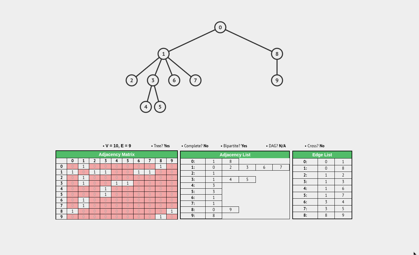
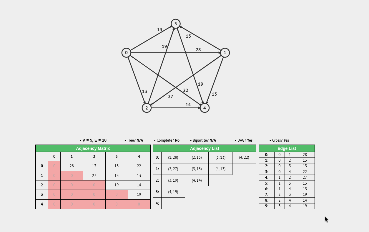
There are three ways to represent a graph in memory:

graph-representation graph-representation2

A 2D array (or grid) of size \(V \times V\) where cells contain edge weights (or boolean values indicating presence).

Pros:

\(O(1)\) Edge Lookup: Checking whether an edge exists between vertex \(u\) and \(v\) takes constant time.
Edge Weight Access: Excellent for dense graphs and algorithms that frequently query weights directly (e.g., Floyd-Warshall).
Simplicity: Straightforward to implement using a standard 2D array or flattened memory block.

Cons:

High Memory Overhead: Requires \(O(V^2)\) space, which becomes extremely wasteful for sparse graphs where \(E \ll V^2\).
Slow Neighbor Iteration: Finding all neighbors of a vertex requires scanning an entire row of size \(O(V)\), even if the vertex has only one connection.

An array or hash map of vertices, where each vertex stores a collection (typically a linked list or dynamic array) of its adjacent neighbors.

Pros:

Space Efficient: Requires \(O(V + E)\) space, making it optimal for sparse graphs (which most real-world graphs are).
Fast Neighbor Traversal: Iterating over the neighbors of a vertex takes \(O(\text{degree}(v))\), which is proportional to the actual number of connections.

Cons:

Slow Edge Lookup: Checking if a specific edge exists between \(u\) and \(v\) requires scanning the neighbor list of \(u\), taking \(O(\text{degree}(u))\) time.
Cache Locality Issues: Depending on implementation (e.g., linked lists), node allocations can scatter across memory, leading to pointer chasing overhead.

Similar to an adjacency list, but each vertex stores its neighbors in a set (such as a Hash Set or Tree Set) instead of a sequential list.

Pros:

Fast Edge Lookup with Sparsity: Retains the \(O(V + E)\) space efficiency of adjacency lists while providing \(O(1)\) average-time edge existence checks (if backed by a Hash Set).
Efficient Vertex Removal: Deleting edges or vertices is faster because sets support \(O(1)\) or \(O(\log K)\) removal without needing to shift array elements or traverse entire lists.

Cons:

Higher Memory Overhead: Hash sets or balanced trees consume more memory per vertex than simple dynamic arrays or linked lists due to load factor buffers and node overhead.
Overhead for Small Degrees: For vertices with very few neighbors, the overhead of a set data structure outweighs its benefits compared to a simple list.

Representation	Space Complexity	Edge Lookup	Neighbor Iteration	Best Used For
Matrix	\(O(V^2)\)	\(O(1)\)	\(O(V)\)	Dense graphs, frequent edge weight queries
List	\(O(V + E)\)	\(O(\text{degree}(v))\)	\(O(\text{degree}(v))\)	Sparse graphs, frequent traversals (BFS/DFS)
Set	\(O(V + E)\)	\(O(1)\) (average)	\(O(\text{degree}(v))\)	Sparse graphs requiring fast edge existence checks